Dijkstra's Algorithm for Shortest Path

Rahul Pandey | May 16, 2017

Dijkstra’s algorithm is a method to find the shortest paths between nodes in a graph. In particular, Dijkstra’s algorithm solves the single-source shortest path problem: find the shortest path from a single node to all other nodes in the graph. We assume in the discussion below that the graph G on which we operate is connected, undirected, and each edge has a nonnegative weight [1]. We can think of the graph as a collection of major cities (nodes) connected by highways of a certain distance (edges).

Contents

• Summary
• Implementation and Runtime
• Variants
• References

Summary

The intuition behind Dijkstra’s algorithm is simple. If we wanted to find the shortest path between two cities A and B, we could just try all possible paths between A and B. Once we arrive at a node, let’s say we can clone ourselves to travel to each outgoing edge. When a clone reaches a node, it checks to see if another clone had already been to that node. If so, the clone stops: this clone was not the fastest to reach the node (therefore, this clone took a longer path). If another clone had not been to the node, this clone’s path to the node was the fastest (and, therefore, the shortest). This is the idea behind Dijkstra’s algorithm, but we use the edge distances instead of time to keep track of the shortest path [2].

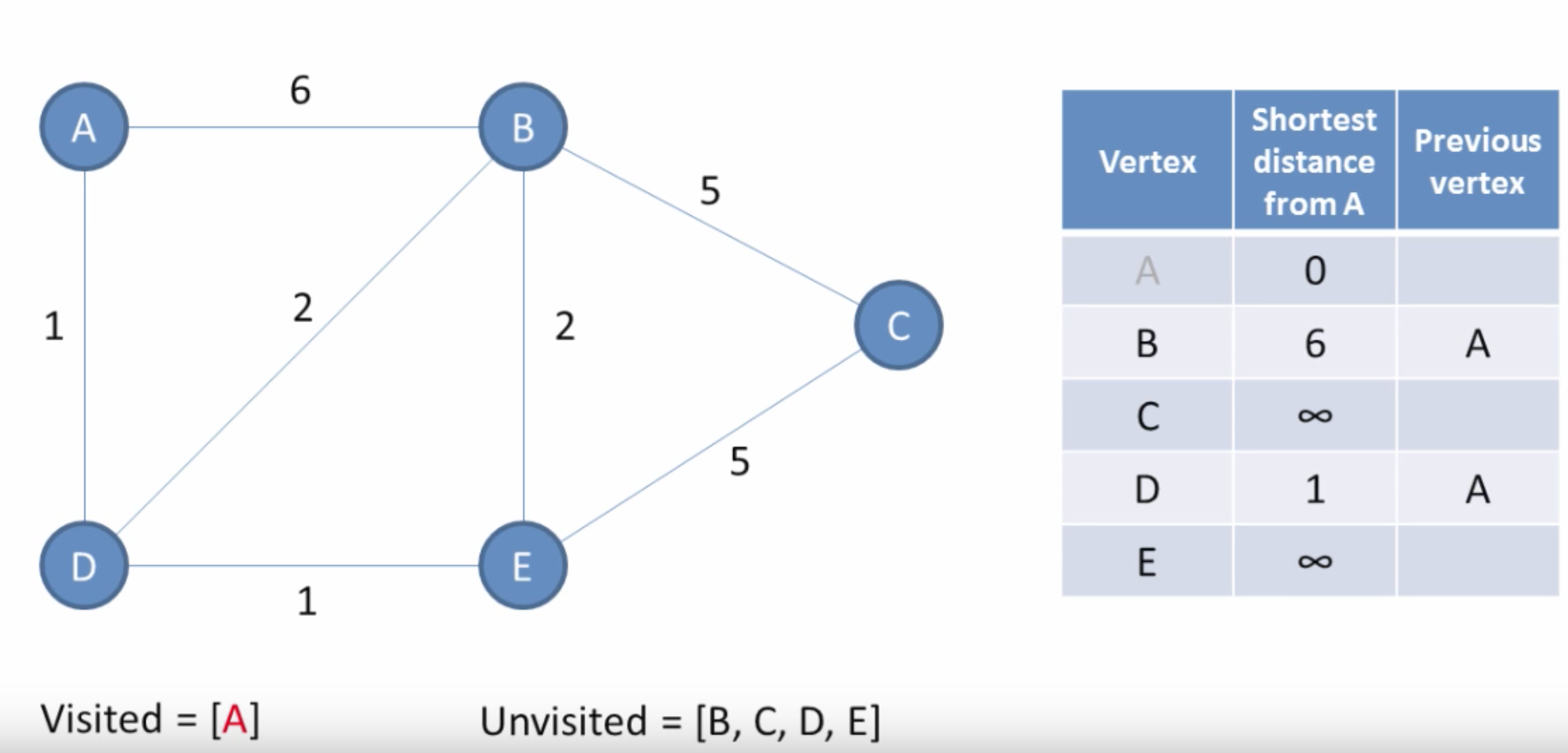
The input to Dijkstra’s algorithm is a graph G and a source node (or root) v. The algorithm works by assigning a cost value to each node and then updating it until it becomes optimal. Initially, the cost of the starting node is 0, and all others are infinity. (Images are from [4].) The algorithm is then:

1. Select a node n from the unvisited nodes which has the least weight.
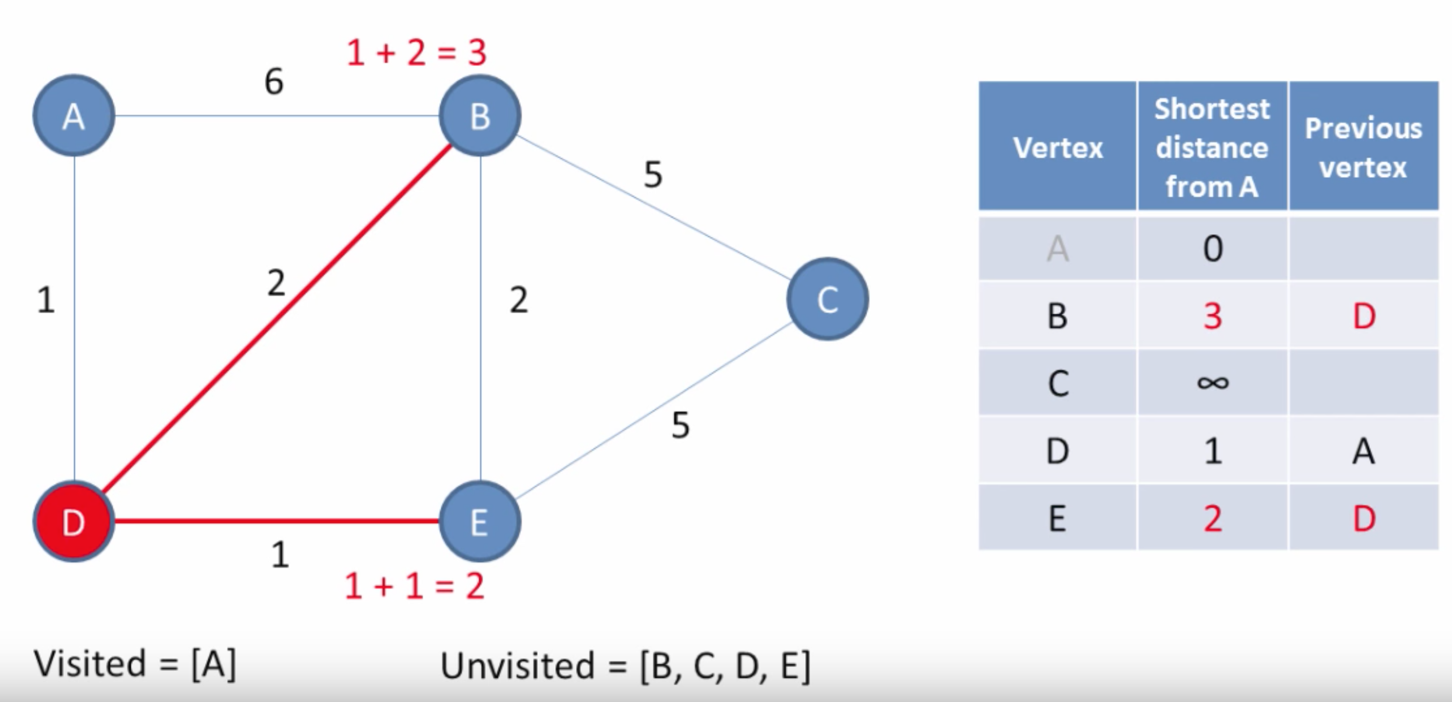
2. For each neighbor x of n, compare path_weight[x] to path_weight[n] + edge_distance[(n, x)]. This is determining, can we get a path from the root to x with smaller distance by going through n instead of the current best path? If so, we update the weight of x to the new distance.
3. Remove n from the set of unvisited nodes.

Starting at the current location, we search for unexplored points, which become candidates for our next location. We figure out the next location by calculating which of the candidate nodes has the least cost path to that node, and in that process we slowly expand the set of visited nodes for which we’ve found the shortest path.

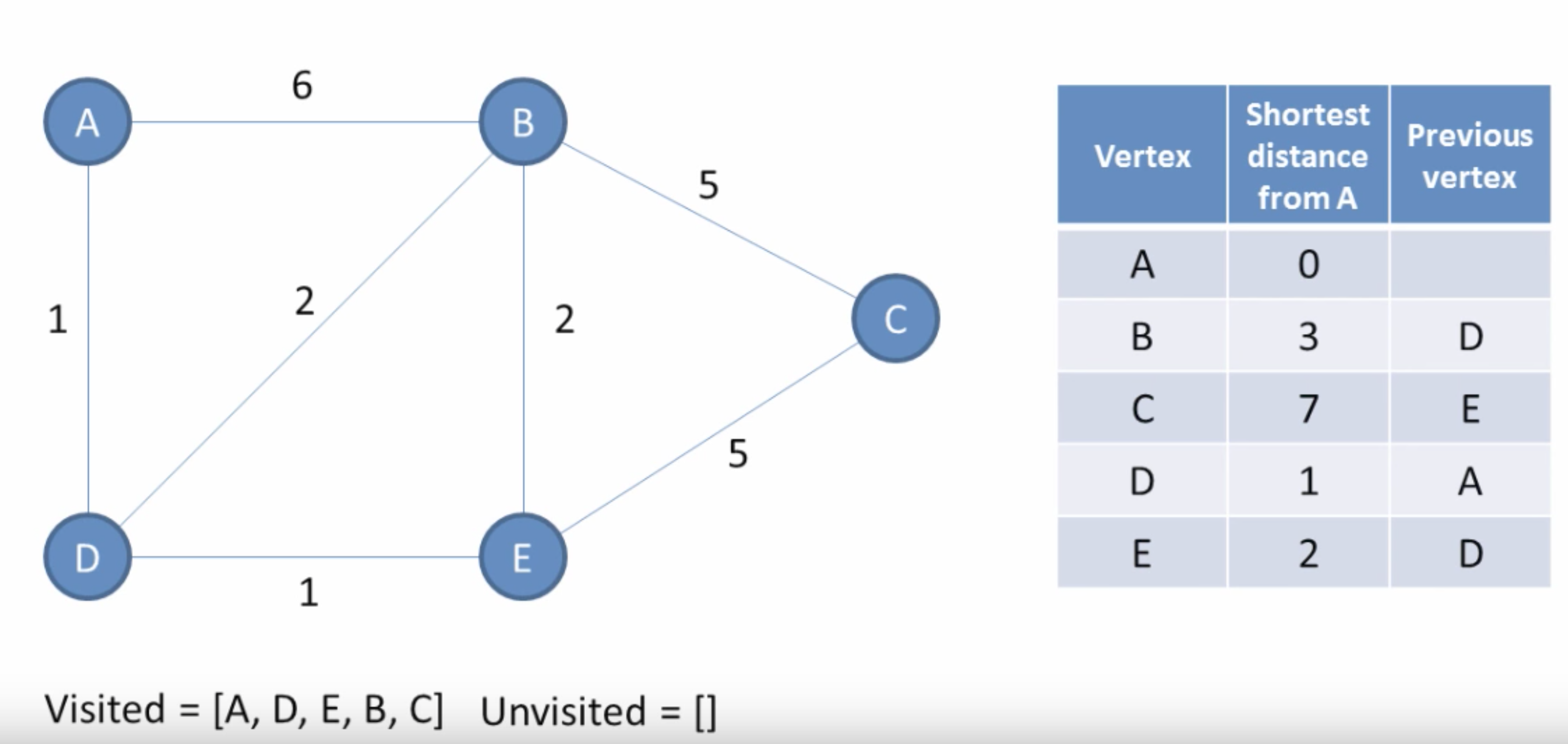
The result of Dijkstra’s algorithm starting at node v is a shortest path tree rooted at v, such that the path from root v to any other node in the tree is the shortest path distance. The shortest path tree is a spanning tree, meaning that it is a subgraph which includes all the vertices of G.

Implementation and Runtime

To pull out the least weight node in step 1 of the algorithm, we use a data structure called a Priority Queue, which allows us to retrieve an object with the minimum associated key. It acts like a queue except that it supports the ability to efficiently extract the highest priority item instead of simply the oldest. Priority queues are often implemented with a heap, so check out that article for more info!

The worst-case runtime of Dijkstra’s is O(|E| + |V| log|V|), where E and V are the edge and node set, respectively. This is because we check each edge of the graph in the traversal, requiring O(|E|) time. We must also pull out each node from the priority queue, where each extract operation takes O(log|V|) time. So the total time is O(|E| + |V| log|V|).

Conceptually, we can think of Dijkstra’s algorithm as breadth-first search where each edge has weight 1. In BFS, since we consider all edges to have the same weight, we can simply use a normal queue instead of a priority queue since the nodes will obey the first-in-first-out (FIFO) ordering.

Variants

Bellman-Ford Algorithm

Unlike Dijkstra's algorithm, the Bellman-Ford algorithm is able to handle negative edge weights. Bellman-Ford is more powerful than Dijkstra's, but it's also slower [3]. The idea behind Bellman-Ford is similar to Dijkstra's in that both use the principle of relaxation: an approximation to the correct distance is gradually replaced by more accurate values until eventually reaching the optimum solution. Instead of using a priority queue, though, Bellman-Ford needs to update the cost for all outgoing edges from a node.

Floyd-Warshall Algorithm

The Floyd-Warshall algorithm finds the shortest path in a graph with positive and negative edge weights, but a single execution of the algorithm finds the shortest path between all pairs of vertices. This is unlike Dijkstra's or Bellman-Ford, which computes the shortest path from a source to all other nodes. The output of Floyd-Warshall is equivalent, for example, to running Bellman-Ford on every node.

What about negative cycles?

Bellman-Ford and Floyd-Warshall are able to operate on graphs with negative edge weights. However, if a negative cycle exists (a cycle whose edges sum to a negative value), then there is no cheapest path; any "shortest" path can be made shorter by walking along the negative cycle. In these cases, the best we can do is report the existence of the negative cycle.

References

[1] Dijkstra’s Algorithm wiki

[2] Dijkstra’s Algorithm in Cracking the Coding Interview

[3] Bellman-Ford Algorithm wiki

[4] Dijkstra’s Algorithm YouTube video